Introduction
Glioblastoma (GBM) is the most aggressive and common type of brain tumour in adults. The main challenges patients face are the low survival rate, extraordinarily high tumour heterogeneity, and lack of specific treatments of GBM [1]. In classic clinical practices, histopathology images are manually analysed by medical experts or pathologists for diagnosis of disease stage [2]. However, manual analysis can cause some problems:
There is no standard assessment for the diagnosis. Experiences and subjectivity of medical professionals or pathologist can impact evaluation criteria significantly [3].
It is a protracted and monotonous task that pathologists visually navigate and review glass slides or whole slide images (WSI) to detect and analyse malformations in daily work [4]. After evaluating the brain graphics, if tumour existence is disbelieved, the patient’s brain biopsy will be activated. Unlike magnetic resonance (MR), biopsy has an invasive process, and sometimes, it may even consume a month to determine an answer [5].
Therefore, the result of the analysis is not quantitative. For these cases, an efficient and quick method of analysing images is urgently needed.
Objectives
The main goals of this research are:
- To establish a computer-based system that can detect and classify different types of tumour cells.
- Finding out the percentage of positive cells to all cells shown in the image.
- Reducing the costs in viewing time, examination and interference from human factors, thereby assisting pathologists to improve the accuracy in clinical diagnosis.
Methodology
Manual extraction of training and validation dataset
Three of 22 whole slide images were randomly selected as testing samples for this research. The rest of images are used to train our network. All cells in these images were extracted and divided into five classes: single positive cells (SP), single negative cells (SN), connected positive cells (CP) and connected negative cells (CN). Also, the background information (BG) was collected as negative samples for the training dataset. Some examples of the training samples are presented in figure 1.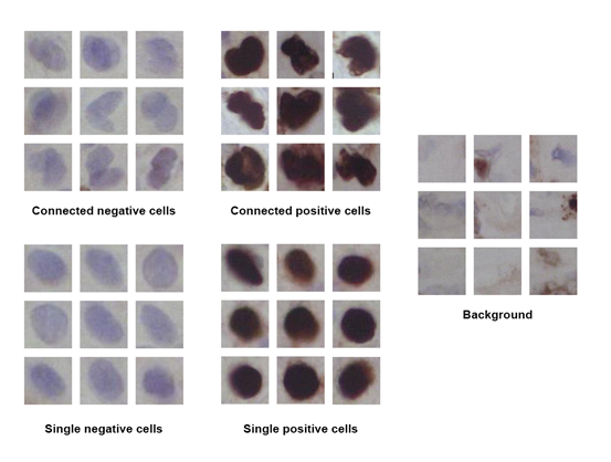 Figure 1-cell classification overview
Deep Residual Network (ResNet) classification
In order to classify different classes of cells based on different sizes of patches from the detector, a popular classifier called ResNet50 [6], was chosen to train on the extracted dataset with stochastic gradient descent (SGD) optimizer, momentum of 0.9, learning rate of 0.002, and cross entropy as loss function.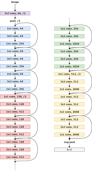 Figure 2, the architecture layout of ResNet50
Cell detection and segmentation
While testing images, cells are detected and identifies by using sliding window with softer non-maximum suppression (NMS) [7]. In addition, the size of bounding boxes has been configurated in advance. All of connected cells identified by trained classifier are then been split into a single cell based on the watershed algorithm. Finally, the detected cells were counted based on their predicted label.
Evaluation criteria
To assess the performance of our classifier, we used precision, recall and F-score as performance measurement matrices derived from true positive (TP), true negatives (TN), false negatives (FN) and false positive (FP) values. Also, we compare the predicted proliferation index that obtained from detection to ground truth and show the difference as error rate.
Precision, recall, F-score and error rate are defined as follows:
$$ Precision=\frac{TP}{TP+FP} $$
$$ Recall=\frac{TP}{TP+FN} $$
$$ F=\frac{2(Recall*Precision)}{Recall+Precision} $$
$$ Error rate=\frac{DL-Munually}{Munually} $$
Results
To make full use of limited datasets and prevent the over-fit, K-fold cross validation was used for training the model. The cells that extracted from original images were split into five subsets before training. Every subset contains 20% of the total data. We performed 50 epochs with 5-fold cross validation to train the model.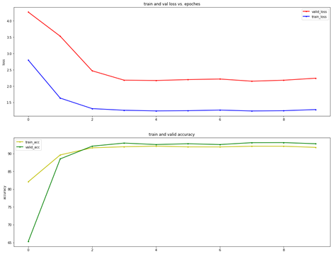 Figure 3 – loss and accuracy vs. the number of epochs
Figure 3 shows the accuracy and loss values in training and validating phase for each 5-fold cross validation. The highest validated accuracy of model reached 93.3%, which was selected as the classifier to recognise cells.
For evaluating performance of the model, we prepared three original-size images (1392×1040 for the size) that are unseen for the model. The result of the assessment has been demonstrated in table 1.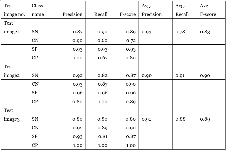 Table 1 – evaluation measure on three test images
Furthermore, a comparison of calculating proliferation manually and based on our trained model has been indicated in the Table 2.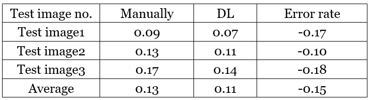 Table 2 – proliferation score concluded by different measures and comparison
Detection time is one of important factors of object recognition. Generally, the algorithm is supposed to keep a high accuracy of detection and complete the task as soon as possible. In our experiment, it took an average of 13 minutes for identifying each image.
Moreover, the cell detection and segmentation algorithm were implemented using Python and OpenCV tools on a machine with AMD 3500X processor, 16GB RAM, NVIDIA RTX2060 GPU.
Conclusion
In this study, we propose an approach combined with deep learning and image segmentation to detect, categorize and count cells in the GBM histological images. The model implemented provides high accuracy and performance according to the result of quantitative evaluation that includes precision, recall and F-score. Compared with manual annotations, the proposed model shows an acceptable error rate of cells recognition.
However, this model still has some shortages. It is time-consuming to detect cells based on sliding window algorithm. Although the time cost can be reduced by increasing step sizes of sliding window, the recall rate of detection will be decreased simultaneously. Also, configured bounding boxes constrict the size of cells that can be detected. If the size of cells exceeds these bounding boxes, the detector may fail. Further studies should concentrate more on optimization of object detection and segmentation. Some new methods, such as CBNet and YOLO v4 should be considered in future research to improve the performance.
Reference
- Lee, E., Yong, R.L., Paddison, P. and Zhu, J., 2018, December. Comparison of glioblastoma (GBM) molecular classification methods. In Seminars in cancer biology (Vol. 53, pp. 201-211). Academic Press.
- Chen, R., Smith-Cohn, M., Cohen, A.L. and Colman, H., 2017. Glioma subclassifications and their clinical significance. Neurotherapeutics, 14(2), pp.284-297.
- Yonekura, A., Kawanaka, H., Prasath, V.S., Aronow, B.J. and Takase, H., 2017, September. Glioblastoma multiforme tissue histopathology images-based disease stage classification with deep CNN. In 2017 6th International Conference on Informatics, Electronics and Vision & 2017 7th International Symposium in Computational Medical and Health Technology (ICIEV-ISCMHT) (pp. 1-5). IEEE.
- Sharma, H., Zerbe, N., Klempert, I., Hellwich, O. and Hufnagl, P., 2017. Deep convolutional neural networks for automatic classification of gastric carcinoma using whole slide images in digital histopathology. Computerized Medical Imaging and Graphics, 61, pp.2-13.
- Anaraki, A.K., Ayati, M. and Kazemi, F., 2019. Magnetic resonance imaging-based brain tumor grades classification and grading via convolutional neural networks and genetic algorithms. Biocybernetics and Biomedical Engineering, 39(1), pp.63-74.
- He, K., Zhang, X., Ren, S. and Sun, J., 2016. Deep residual learning for image recognition. In Proceedings of the IEEE conference on computer vision and pattern recognition (pp. 770-778).
- He, Y., Zhang, X., Savvides, M. and Kitani, K., 2018. Softer-nms: Rethinking bounding box regression for accurate object detection. arXiv preprint arXiv:1809.08545, 2.


- 本文链接:http://yoursite.com/2020/12/06/Research_UROS/
- 版权声明:本博客所有文章除特别声明外,均默认采用 许可协议。
若没有本文 Issue,您可以使用 Comment 模版新建。
GitHub Issues